by Nicholas Martens
Nominated by Ana Reynoso for ECON 495: Seminar in Economics: Gender and the Labor Market
Instructor Introduction
Nicholas Martens’ (Nick) paper investigates which type of institutions are most effective at coping with the effects of local labor demand shocks and prevent their residents from migrating out to more favorable labor markets after graduation. Nick uses very detailed microdata from LinkedIn profiles that he impressively collected himself after securing reliable networks during a summer internship. On top of this, Nick employs frontier econometric methods to estimate the impact of demand shocks on the brain drain. This paper, which Nick turned into his Honor’s thesis, is comparable to the best papers we see in the Third Year Paper class for Economics PhD. students, in which graduate students write an original research paper (for most of them, their first experience doing so). Because Nick’s paper checks all the boxes of an exemplar paper for my ULWR class, I invited him to be a guest speaker for the next cohort of the class and he gave a wonderful summary of the comprehensive process of making this impressive paper.
I have no doubt that this paper will be extremely well published because it advances the frontier of knowledge in significant ways. In fact, one of the prominent authors in the literature---a Michigan alum, now a professional researcher---came to give a full seminar on his related work in progress and I found myself referring this speaker to Nick’s class paper during his seminar. I mentioned Nick’s paper as an example of related work that has the right data to overcome many of the empirical issues the presenter was talking about.
I am more than honored to have advised Nick’s paper which is very well deserving of this highly competitive Sweetland Writing Prize. I am sure we will see great things from Nick as he progresses in his career.
— Ana Reynoso
Plugging the [Brain] Drain
Evidence from the LinkedIn profiles of college graduates
1 Abstract
Concentration of educated workers presents economic and political challenges, namely regional economic divergence and mounting political polarization. Likewise, colleges and universities face increasing pressure to stimulate local economic growth in addition to educating students. Arguably, no metric matters more for an institution’s local economic impact than the retention of graduates within the state or local labor market. Characteristics like selectivity, research intensity, and institutional control significantly affects the probability of graduates returning to the labor market and state containing their high school. Given the growing interest in mitigating brain drain and institutional effects in higher education, my research helps policymakers discern which institutions produce graduates who reside in their communities after receiving a bachelor’s degree.
I use data from individual LinkedIn profiles to answer the research question. Since LinkedIn users list the time and location of positions, I treat it as migration microdata. Further, LinkedIn profiles include educational attainment and the institution where they obtained each degree. I cannot mitigate the problem of individual identification, precluding establishment of causal mechanisms. Instead, I conduct descriptive analysis with the LinkedIn profiles.
Local labor demand is my independent variable, measured with County Business Patterns data aggregated to the labor market level. I measure local labor demand with the Bartik instrument, which interacts cross-sectional differences in industrial structure with national employment growth by industry. The dependent variable is a binary variable for individuals, indicating whether they returned to their high school labor market or state within 10 years of college graduation.
2 Introduction
In May 2023, urban scholar Richard Florida gave a speech to policymakers in Michigan where he said:
“You’re using Michigan taxpayer dollars to subsidize the coastal high-tech economy. Now, if I’m a youngster coming out of University of Michigan, Wayne State, Michigan Tech, MSU. I want a good job and a good place. So [we’ve got them] drifting for San Francisco or New York or wherever...I think I need to think about that and what would it take to keep them.” (Davidson, 2023)
Public research universities, especially the University of Michigan and Michigan State University, dominate public perceptions of higher education in Michigan, reinforced by high-profile athletic events, academic prestige, and robust alumni networks. In Michigan, recent media coverage of brain drain and policy initiatives focus on the state’s public research universities (Growing Michigan Together Council, 2023; French, 2023; LeBlanc, 2023a; LeBlanc and Hall, 2023). Yet the most prominent avatars for public higher education are generally least effective at producing graduates who stay after graduation. Indeed, Michigan Tech, the University of Michigan and Michigan State rank second, third and fourth respectively among Michigan’s 15 public universities in share of graduates moving out-of-state (Conzelmann et al., 2022; French, 2023). Michigan hosts fifteen public universities, though Florida only mentioned four, all with substantial research activities. Florida’s choice of institutions reflects a larger focus among policymakers in retaining graduates of Michigan’s most prestigious research universities. Shortly after Florida’s speech, Governor Gretchen Whitmer formed the Growing Michigan Together Council to catalyze Michigan’s sluggish population growth (LeBlanc, 2023b). The proposals in the Council’s first report broadly affect Michigan’s post-secondary education system, particularly regional universities most reliant on in-state and transfer students (Growing Michigan Together Council, 2023). Yet the report only references three institutions by name: Wayne State, Michigan State, and the University of Michigan (Growing Michigan Together Council, 2023; LeBlanc, 2023a,b). Policymakers’ focus on prestigious research universities raises the question: why do graduates of research universities leave at higher rates than graduates of other institutions? This paper explores how institutional characteristics affect migration behavior of graduates using data from LinkedIn profiles. Much of the analysis focuses on public universities, delineating between large research-intensive flagship institutions and regional public universities (RPUs) with greater emphases on undergraduate education. Graduates of flagship institutions leave their high school labor market at significantly higher rates than RPU alumni.
2.1 Labor Shocks and Migration
People often live near their childhood home. Thirty percent of Americans born between 1984 and 1992 live in the same Census tract at ages 16 and 26, while 58 percent reside within ten miles of their childhood home (Sprung-Keyser et al., 2022). Most people esteem local ties, deriving high utility from their network of friends and family (Zabek, 2019). The attachment to place persists during economic downturns, driving down real wages and lowering labor force participation rates. Hershbein and Stuart (2022) find out-migration rates fell in labor markets with the most severe employment declines during recessions. Instead, lower rates of in-migration drive population losses in communities with steep employment declines. In many cases, the appeal of local social networks blunts the effects of adverse labor market conditions.
While amenities likely figure into most people’s utility functions (Florida, 2002), labor market conditions heavily inform migration decisions for college graduates (Conzelmann et al., 2022; Wozniak, 2010; Bound and Holzer, 2000; Notowidigdo, 2020). People with post-secondary education are more likely to reside in states with positive labor market conditions when they were in their twenties (Wozniak, 2010). College graduate settlement patterns yield important ramifications for the cohesion of the United States, given the outsize role migration plays in regional economic divergence.
2.2 The Problem of Educational Sorting
College graduates increasingly live in different metropolitan areas than non-graduates, with the disparity growing over the last four decades (Diamond and Gaubert, 2022; Diamond, 2016). College graduates provide benefits to the communities they inhabit, including social benefits like lowered crime and improved health outcomes (Moretti, 2003). Locales with higher proportions of college-educated workers enjoy stronger productivity and wage growth for all workers, regardless of educational attainment (Diamond, 2016). Yet in-migration of educated workers endogenously improves amenities, boosting the well-being of educated workers relative to less-educated ones (Diamond, 2016). Diamond and Moretti (2021) observes a strong negative relationship between consumption and prices for non-college households, but no relationship for college-educated ones. The college wage premium allows educated workers to maintain or boost consumption in high-cost metros, but workers without college degrees must cut consumption in expensive, ’superstar’ metros (Diamond and Moretti, 2021). Accordingly, high-cost coastal areas like Washington, California, New York, and the District of Columbia are net importers of college graduates, while nation’s interior exports graduates (Conzelmann et al., 2022). Spatial clustering of educated workers worsens inequality across the country and within the migration destinations of educated workers.
The clustering of college graduates accelerates regional economic divergence, entrenching regional winners and losers within the United States. Regional economic divergence defies the spatial convergence predicted by standard economic frameworks like the Rosen-Robeck model (Roback, 1982). Technological advancement and de-industrialization remain the dominant economic explanations (Autor et al., 2013). Institutional changes over the last four decades, such as weakened antitrust enforcement and increased competition between local governments for economic development, potentially exacerbate regional economic divergence (Manduca, 2019; Pacewicz, 2016). Economic divergence gnaws at national cohesion, complicating the work of national policymakers constrained by a single budget and interest rate (Manduca, 2019). As college graduates cluster, regional inequality across the United States worsens, contributing to political polarization (Autor et al., 2020) and wide variation in social mobility (Chetty et al., 2014).
From the perspective of taxpayers, the clustering of college graduates generates spatial variation in the return on investment for public higher education (Conzelmann et al., 2022). Across the United States, high-wage urban areas retained more college graduates per dollar invested in higher education. Locales that import college graduates enjoy more of the social benefits wrought by college graduates (Conzelmann et al., 2022). Importantly, migration behavior varies substantially by institution. Conzelmann et al. (2022) find selective RPUs generate greater returns on public investment than flagship universities, driven by alumni populations with less spatial mobility. In short, institutional characteristics matter as policymakers rectify the spatial concentration of college graduates.
2.3 Institutional Effects
The United States contains thousands of institutions granting bachelor’s degrees, serving more than 15 million students (National Center for Education Statistics, 2022). Unsurprisingly, undergraduate experiences and post-graduation outcomes vary by institution. Post-graduation earnings trajectories, occupational profiles, spatial distribution, and socioeconomic composition differ greatly by institution type (Chetty et al., 2020; Conzelmann et al., 2022). Socioeconomic inequality drives some of the variation in outcomes. American higher education segregates by class, with students from top fifth of the income distribution 77 times more likely to enroll at elite institutions than those from the bottom fifth (Chetty et al., 2014). Despite intra-institution segregation by class, low-income students who attend elite institutions enjoy the same earnings trajectories as their peers from wealthier backgrounds (Chetty et al., 2020). In other words, post-secondary institutions facilitate movement across social classes. Parental income also shapes migration patterns. Sprung-Keyser et al. (2022) finds a clear relationship between parental income and probability of relocation: as parental income increases, children are more likely to relocate to distant commuting zones as adults. Perhaps unsurprisingly, idiosyncratic structures like alumni networks and university career centers potentially contribute to the spatial concentration of college graduates, at least among alumni of elite universities (Manduca, 2022). Despite the outsize role institutional characteristics play in migration of college graduates, literature exploring institution types and brain drain remains sparse.
Data limitations contribute to the paucity of literature. Limited data linking workers to hometowns constrains the literature on the relationship between hometown and migration preferences (Dahl and Sorenson, 2010; Carr and Kefalas, 2010; Sprung-Keyser et al., 2022). The sample tracked by Sprung-Keyser et al. (2022) only includes educational attainment for individuals who responded to the American Community Survey (ACS). Earlier analyses suffered even greater limitations. Most rely on five percent samples of the Decennial Censuses or the ACS, depending on the years of analysis (Diamond and Gaubert, 2022; Wozniak, 2010; Bound and Holzer, 2000). Neither the ACS nor the Decennial Census samples include birth or migration data at any level more granular than the state, precluding exploration at a more detailed spatial level.
Large national surveys may collect data on institution and migration, though LinkedIn sample sizes are scales of magnitude larger, allowing for greater geographic coverage. The Panel Study of Income Dynamics asks respondents about where they attended college, but geolocation and secondary school data are restricted-access only. Likewise, the National Longitudinal Survey includes a migration distance variable, though data isn’t as reliable as state and county of residence variables. The Census Bureau’s new Post-Secondary Employment Outcomes (PSEO) dataset offers promise, though coverage varies greatly by state and sample sizes remain small (Conzelmann et al., 2022). For example, the only institution in Michigan included in PSEO is the University of Michigan–Ann Arbor. By contrast, LinkedIn enables analysis of sub-state migration matters and characteristics of post-secondary institutions.
College graduates exhibit greater spatial mobility than people without bachelors degrees (Wozniak, 2010; Bound and Holzer, 2000). Using LinkedIn data, Conzelmann et al. (2022) find graduates of more selective institutions travel further and exhibit greater dispersion. However Conzelmann et al. (2022) relies on summary data by institution, rather individual-level microdata linking high schools, colleges, and post-graduation outcomes. Due to data constraints, limited research contextualizes post-college migration decisions with hometowns. Given the importance of local ties in shaping migration decisions, analyses of migration that exclude origin data likely suffer from omitted variables bias (Zabek, 2019; Hershbein and Stuart, 2022).
Adapting the empirical strategy in Notowidigdo (2020) and Bound and Holzer (2000), I use a Bartik instrument to estimate local labor demand shocks. Wozniak (2010) also employed the Bartik instrument to assess the entry conditions of young workers into local labor markets. The instrument projects local employment growth based on national employment growth and local industrial mix, constituting the independent variable (Bartik, 1991). Thus, the instrument delineates employment growth stemming from supply factors and global shifts in demand. Return to high school labor market (or state) within 10 years of college graduation is the dependent variable. I want to see whether selectivity affects the probability of a college graduate residing in the locality containing their high school.
3 Theoretical Framework
I adapt theoretical frameworks from Wozniak (2010) and Sprung-Keyser et al. (2022). To understand how individuals make decisions about relocation, consider how they weigh the costs and benefits of moving (Wozniak, 2010). Let C be a set of locations, where individual i inhabits one such location j and considers k a potential destination 1. Individual i belongs to some educational group e, which correlates with human capital. The econometrician cannot directly observe human capital, only its correlates like baccalaureate institutional characteristics or educational attainment (Sprung-Keyser et al., 2022). Let the model include two time periods: {t0, t1} ∈ T . The choice problem is the following:
where U (ωk) is the utility individual i derives from inhabiting location k and e represents an educational group. Education group correlates with human capital. Wozniak (2010) operationalized e as educational attainment. By contrast, I use institutional groupings based on selectivity, flagship status, and control as the basis for e.
Individuals in each educational group expect different wages so E[w(e)kt] is the average wage of education group e in location k at time t. Economic theory predicts a relationship between wages and labor demand shocks: positive demand shocks will boost wages and negative ones will diminish wages (Bartik, 1991). Pkt is the price level at location k at time t, Thus, E(w(e)kt ) / Pkt measures real wages for educational group e in location k at time t.2
Individuals face both recurring and one-time moving costs (Wozniak, 2010), represented by r(e) and o(e) respectively. Assume r(e)jk = o(e)jk = 0 when j = k, so individuals bear no moving costs for remaining in the same location. One-time moving costs consist of expenses typically associated with physical relocation, like beer and pizza for movers, truck rental, and boxes. Recurrent moving costs include the psychological cost of being far from friends and family, return travel costs, and preferences for local amenities in j (Sprung-Keyser et al., 2022). Thus, the costs depend entirely on subjective considerations like individual preferences towards proximity to family, and local ameni- ties. As a result, measurement of recurrent moving costs isn’t possible from existing public data. However, LinkedIn profiles listing high school and college offer a means of (imperfectly) estimating recurrent moving costs. Social ties drive attachment to place, and educational institutions facilitate the formation of social ties (Zabek, 2019). If an individual is attached to a place, the location is likely the site of either secondary or post-secondary educational experiences. Secondary schooling garners particular importance because most people reside with their parents during high school, an effective proxy for familial ties. Thus, I can estimate recurrent moving costs based on the locations of an individual’s high school and college. Educational experiences shape the spatial arrangement of an individual’s social ties, a substantial component of the recurrent moving costs in migration decisions.
According to the model, individual i seeks to live in a location that maximizes utility relative to all other locations, after accounting for moving costs. Put another way, individuals who relocate must satisfy the inequality:

For an individual to relocate, their destination must offer a higher wage, even after accounting for fixed and one-time moving costs. The framework helps explain why domestic out-migration is relatively uncommon (Zabek, 2019; Hershbein and Stuart, 2022). Preferences for one’s current location j embedded in c(e)jk raise the cost of moving. As a result, widespread out-migration requires paltry wages or strong attachment to the labor market. High rates of out-migration among low-income workers in Appalachia satisfy the first condition, driven away due to low equilibrium wages (Sprung-Keyser et al., 2022). The second condition is the focus of the paper. In general, college graduates migrate at higher rates than their peers without college degrees, suggesting college strengthens attachment to the labor market at the expense of place (Notowidigdo, 2020; Wozniak, 2010). I want to know whether institutional characteristics like selectivity, flagship status, and control are salient parameters in migration decisions.
1 For the purposes of my analysis {j, k} are sub-state labor markets and C is the United States
2 Yagan (2014) notes individuals move for two reasons. Some migrate for better labor market opportunities, while others migrate to weaker labor markets to enjoy a lower cost of living. By treating relocation decisions as a function of real wages, I implicitly account for spatial variation in the cost of living.
4 Empirical Strategy
I can operationalize my research question by treating local labor demand as exogenous and residence in the high school labor market (and state) as the dependent variable. I am particularly interested in the effect baccalaureate institution selectivity plays in migration patterns.
4.1 Model
I measure up to 41 years of post-graduation migration behavior, constrained by the time horizon of County Business Patterns from Eckert et al. (2021). Ultimately, the early extent of the time horizon matters little. Figure 4 shows that half of the analytical sample graduated from college in the last 10 years. The first decade after college graduation heavily influences long-term settlement decisions (Wozniak, 2010). Less likely to be constrained by complex familial considerations, Americans exhibit the most mobility in their twenties, when most people obtain post-secondary credentials (Wozniak, 2010).
I index observations by the labor market of the high school, denoted by j. Importantly, only the high school needs to be in j; the college can be anywhere in the United States. However, people who stay in the same labor market for high school and college (j = k) face a different decision-making process than people who leave their high school labor market for their bachelor’s degree (j ̸= k). People who attend college elsewhere compare the conditions of their home labor market j relative to their college labor market k. Those who stay cannot make such a comparison. Their decision to remain depends on the conditions of the labor market where they attended both college and high school. Equation 3 below describes the return rate as a function of local economic conditions in the labor market of the high school j and college k if j ̸= k:
stayij = β1hsLDjt + β2colLDkt + β3colType + β4(colType × si) + βX′ + ϕM + αt + µijt (3)
where stayij is a binary indicator for individual i ever residing in their high school labor market j (or state M ) at any time t ∈ T after college graduation such that
stayij =
1 Individual i attended high school in labor market j and resided in labor market j at a time t ∈ T
0 Individual i attended high school in labor market j and never resided in j at a time t ∈ T
hsLDjt is the labor demand shock at time t in the labor market j containing the high school,
colLDkt is the labor demand shock at time t in labor market k containing the college,
colType is the grouping of the baccalaureate institution, described more in Section 5.3
si =
1 Individual i received bachelor’s degree from institution in same state as high school
0 Individual i did not receive bachelor’s degree from institution in same state as high school
X′ i is a vector of individual controls: transfer status, age at bachelor’s attainment, and major
ϕM measures fixed effects in state M containing high school labor market j such that j ⊆ M
αt reports proportional shocks across all labor markets in a given time period, and
µijt captures unobservable error.
For a more detailed explanation of identification issues, go to The Problem of Individual Identification. The null hypothesis supposes every individual i graduating from a high school in labor market j has the same probability of living in j at time t after graduating from college.
4.2 Bartik Local Labor Demand Instrument
I use the Bartik shift-share instrument to estimate local labor demand variables hsLDjt and colLDkt (Bartik, 1991). The Bartik instrument enables direct comparison of labor demand shifts of equal magnitude but opposite sign (Notowidigdo, 2020). Both Wozniak (2010) and Bound and Holzer (2000) employ the Bartik instrument to gauge the relationship between local labor market conditions and migration.
4.2.1 Assumptions
Importantly, Bartik instruments assume no correlation between national employment growth by industry and local labor supply shocks (Bartik, 1991). Thus, the instrument detects “plausibly exogenous” (demand-induced) variation at the commuting zone level (Notowidigdo, 2020). Further, the model in Equation 3 assumes that the instrument does not correlate with unobserved shocks in the local labor supply (represented by ϵ).
4.2.2 Formal Definition
The Bartik instrument interacts cross-sectional differences in industrial structure with national changes in employment growth by industry (Goldsmith-Pinkham et al., 2020). The formal definition begins by calculating predicted employment change πi,t, below:

where i indexes commuting zones, t indexes time periods, k indexes industries ∈ K. Let τ represent the time period for measuring change such that t−τ represents the start of the period and t marks the end of the period. Thus, γi,k,t−τ records the share of local employment in industry k at time t − τ . The Bartik instrument measures national industry employment growth rates vk,t − vk,t−τ . Since national shifts do not require summation at the commuting zone level, vk,t does not use the commuting zone index i. The instrument then calculates predicted employment change between time t − τ and t:
Eˆi,t = (1 + πi,t)Ei,t−τ (5)
where Ei,t−τ consists of total local employment at time t − τ and (1 + πi,t) converts predicted employment change to a ratio. The proxy for labor demand appears below:

where Ei,t−τ remains local employment at time t−τ and Eˆi,t records the employment total predicted by the instrument for time t. Thus, ∆θˆi,t is the difference between predicted and actual employment, divided by the actual employment at time t − τ .
Thus, the results in subsequent sections of the paper estimate demand using ∆θˆ for two local labor markets: j containing high school and k containing baccalaureate institution.
∆θˆj,t = hsLDjt (7)
∆θˆk,t =colLDkt (8)
5 Data
Equation 3 combines four types of data: geographic and demographic data from LinkedIn profiles, secondary and post-secondary institutional characteristics from the National Center for Education Statistics, Barron’s selectivity ratings, and labor demand shocks estimated with County Business Patterns data.
5.1 LinkedIn
I created a database of individual-level educational attainment and migration behavior using LinkedIn profile data. Revelio Labs pulled the data, then the Brookings Institution’s Workforce of the Future Research Initiative provided access to the data. Each profile includes information on:
- Which high school individual an attended
- Which college an individual attended
- Where an individual lived post-graduation
LinkedIn is not a representative sample of the labor market, so I focus on working-age college graduates best represented in the data, imposing the following restrictions on the dataset:
- Graduated from college 1982-2021
- Bachelor’s degree
- High school degree
- At least one job after college graduation with a location listed
Since I wanted to focus on domestic migration patterns, I omitted individuals who attended college or high school outside the United States. Users need to list at least one position after their college graduation in the United States. This paper relies on a sample from seven states. 3
3Delaware, Kansas, Maine, Mississippi, Nevada, New Hampshire, South Dakota

5.1.1 Resumes as Migration Microdata
A LinkedIn profile that includes a high school, college, and some post-graduation work experience tells a story missed by standard survey data like the American Community Survey or even administrative data from the IRS. LI links degrees to educational institutions and employment to spatially-defined labor markets. In other words, LI provides a record of the educational institution an individual attended and residential choice post-graduation.
The two most common methods for exploring migration, ACS microdata and Decennial Census samples, suffer from limitations. The ACS asks respondents about the field and degree obtained, but not the institution. The five percent Decennial Census samples remove any possibility of sub-state analysis, since states are the most granular geography describing birthplace and residence in the microdata. Like the ACS, the samples from Decennial Census also lack data on the characteristics of baccalaureate institutions. By contrast, LinkedIn enables analysis of sub-state migration and characteristics of post-secondary institutions.
5.1.2 Demographic Representation in LinkedIn Profiles
Of course, LinkedIn suffers from limitations (Kreisman et al., 2021). Crucially, self-reporting of educational experiences leads to systematic under-reporting of certain educational experiences, namely non-completion of degrees. Despite accounting for nearly half of all college attendees and roughly one-third of workers, non-completers often hide their post-secondary education. Individuals who attended for less than two years or attended non-selective institutions omit educational experiences at the highest rates (Kreisman et al., 2021). LinkedIn users skew young and college-educated (Conzelmann et al., 2022). Nonetheless, the sheer size of the user population offers research opportunities.
5.1.3 Cleaning and Discarding Observations
Not all LinkedIn profiles contain the same quantity of data. Culling the dataset of profiles with limited information improves the quality of the remaining observations. Most importantly, users must include a high school and a college in the United States. Less than ten percent of college graduates include a high school, and future research should explore whether those who omit high schools may skew towards selective schools and globalized industries. For the current analysis, I impose the following restrictions:
- Graduated from college 1982-2021
- Bachelor’s degree listed in profile
- High school name listed in profile
- At least one job after college graduation with a location listed
Table 1 documents the effect of each restriction on sample size. Since I wanted to focus on domestic migration patterns, I omitted individuals who attended college or high school outside the United States. Users need to list at least one position after their college graduation in the United States with a start date before the end date. While it might seem trivial, some users list jobs with start dates after end dates.
Table 1 indicates that the first restriction imposed (requiring college graduates to include a high school) proves most costly to sample sizes. Given the importance of the restriction, I compare high school includers and omitters in greater detail.
| Reason | Sample |
All BA Completers in US |
1, 420, 546 |
Include HS |
108, 181 |
Work history has geodata |
106, 467 |
Work history has end date after start |
105, 722 |
Work history has start or end date |
105, 706 |
Work history between 1975 and 2023 |
90, 401 |
College appears in IPEDS |
87, 277 |
Graduated college [1982,2021] and born [1930,2002] |
78, 068 |
Educational institutions in 50 states or DC |
78, 066 |
Final analytic sample |
78, 066 |
Table 1: Effect of data cleaning on sample size. Most LI users omit their high school, eliminating more than 90 percent of users. Imposing the requirement of at least one position with a location, start date, and end date removes users with minimal information on their profiles. Availability of County Business Patterns data from Eckert et al. (2021) and the US Census Bureau resulted in the restrictions on college graduation. County-level estimates of labor demand shocks are only available until 2021. Most of the observations removed from the sample were people who graduated after 2021. The limits on estimated year of birth remove obvious outliers that likely stem from data entry errors, like two users allegedly born in 1882 but graduating from college in 1997.
Age Figure 3 depicts the proportion of college graduates who include a high school, by number of years since graduating college. For the first 20 years after college graduation, the proportion of LI college graduates including a high school hovers around 1.8 percent. The proportion of includers continues to rise, peaking for users more than 30 years removed from college graduation. LI users three decades removed from their college graduation were twice as likely to include a high school on their profile as users within two decades of obtaining a bachelor’s degree.
Importantly, few LI users are more than 20 years removed from their college graduation. Figure 4 shows that 25 percent of users graduated from college before 2003. Given the relative youth of the LI user base, the spike in the later years of Figure 3 describes a small subset of users. Thus, the differential reporting of high school by age has a modest effect on the age distribution of the sample. Table 2 reports the age distribution of LI users who omit or include high schools. Omitters are slightly younger though the 10th, 25th, 50th, 75th, and 90th percentiles are within two years of the respective values for includers. With respect to age, inclusion of high school appears random among the younger workers who comprise the bulk of LI users.
Geography Next, I test how geography affects the inclusion of high school on a LI profile. LI users make strategic decisions when they include information on their profile. The inclusion of high school might offer more benefits in smaller labor markets where employers and coworkers live in close proximity.


| Percentile | 10 | 25 | 50 | 75 | 90 |
| HS Includers | 1968 | 1977 | 1988 | 1994 | 1997 |
| HS Omitters | 1970 | 1979 | 1989 | 1994 | 1998 |
Table 2: Age distribution of LinkedIn users who omit and include high school on their profile
| inclusionj | |
| log(totaluserj) | −0.01851 (0.02600) |
| R2 | 0.00005 |
| Adj. R2 | −0.00005 |
| Num. obs. | 10108 |
| ∗∗∗p < 0.001; ∗∗p < 0.01; ∗p < 0.05 | |
Table 3: LinkedIn users are less likely to include their high school in larger labor markets, though the coefficient estimate is not significant. The magnitude of the point estimate is roughly half of the standard error, meaning the coefficient is quite close to 0 given the sample.
Table 3 shows the result of a simple population-weighted regression:
inclusionj = β0 + β1 log(totalusersj) + µj (9)
where j indexes the local labor markets described in Figure 1, inclusionj is the proportion of LI users in labor market j including a high school on their profile, and log(totalusers) is the total number of LI users within labor market j. Congruent with the hypothesis of omission in larger labor markets, β1 is negative. However, the coefficient is not significant, suggesting the negative relationship between high school omission and labor market size could be nothing more than noise.
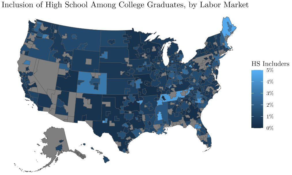
Figure 2 depicts the proportion of college graduates including high school on their LI profile, by labor market. Congruent with the results of the regression, no urbanity gradient seems obvious from the map. While some regional pockets, such as the Mid-South and northern New England, exhibit unusually high rates of high school inclusion, the choice to include high school does not appear to systematically vary with space. Thus, omitting users without LI should not worsen LI’s existing spatial biases.
5.1.4 Linking Educational Experiences to NCES Data
LinkedIn users provide a high school name but not a location, meaning I must guess the location of the high school. In most cases, the name denotes a single school, with one location. Unfortunately, roughly one-third of high schools in the United States have the same name, so the name leaves so ambiguity regarding the home labor market. In these instances, I calculated the distance between the centroid of the user’s college ZIP code and the centroids of potential high school ZIP codes. I keep the high school with the minimum distance. Colleges proved more straightforward for matching. In some cases multiple colleges exist, though matching on college name and state ameliorated any issues.
5.1.5 Estimating Age with Graduation Dates
If someone included a graduation date from high school college, I subtracted 18 to estimate birth the year. Compared to other graduation dates, high school graduations are the best predictor of age because most graduates are 17 or 18. By contrast, more than 27 percent of first-time full-time students who entered college in 2014 graduated in more than four years, accounting for roughly one-third of all graduates from the cohort. Clearly, college graduation dates vary more than high school graduations for a given age cohort. I avoided using graduation dates by taking the start year of a bachelor’s degree included on LinkedIn. For first-time full-time students, start dates should not exhibit such wide variation. If a user includes a bachelor’s degree with a start year, I subtracted 18.
If individuals attended multiple institutions in the United States for bachelor’s degrees (i.e. transfer students), I estimate age using the start date of the earliest institution and measure post-graduation behavior based on the end date of the latest institution.
5.1.6 The Problem of Individual Identification
In addition to inherent issues with self-reported data, LinkedIn data precludes individual identification. Establishing causal mechanisms requires apples-to-apples comparisons between individuals, whether on scholastic aptitude, socioeconomic status, or another basis. LI simply lacks sufficient granularity at the individual level to permit causal analysis, without augmentation from another data source.4
For example, Andrews et al. (2022) measure post-graduation labor market outcomes by major for students of Texas two- and four-year institutions using Texas Education Research Center data, which include academic transcripts and standardized test scores.
For my purposes, I anticipate producing a descriptive analysis of the research opportunities presented by the data. I do not anticipate establishing causal mechanisms, owing to the problem of individual identification.
4Plenty of alternative sources data exist, though few (if any) would trust a 21-year-old with their data.
5.2 Educational Institution Characteristics
The National Center for Educational Statistics at the US Department of Education centralizes data on secondary and post-secondary institutions in the United States.
5.2.2 Secondary Institutions
I obtained data on private and public secondary schools through the 2020-21 Education Demographic Geographic Estimates program, which provides school-level enrollment and geodata. The public school file included enrollment by grade. I excluded any institutions with 0 enrollment in grade 12, namely elementary and middle schools.
5.2.3 Post-Secondary Institutions
I used the Integrated Post-Secondary Education Data System (IPEDS) for post-secondary data. The 2021 Institutional Characteristics Complete Data File includes geodata, enrollment, Carnegie classifications, public status, and myriad other useful variables at the branch (not system) level. I excluded schools that did not offer a bachelor’s degree according to the 2021 data.
5.3 Institutional Groups
I develop a distinct institutional classification system based on selectivity, flagship status, and institutional control.
5.3.1 Barron’s Selectivity Index
Emulating earlier scholarship, I partition post-secondary institutions using Barron’s selectivity index, among other measures (Chetty et al., 2020; Deming et al., 2015; Conzelmann et al., 2022). Barron’s data is not perfect: the cutoffs between institutional groups are arbitrary and perhaps overly reliant on standardized testing. Nonetheless, the ratings capture a notion of academic prestige that profoundly affects American higher education. When possible, I used the replication data from Chetty et al. (2020), available on the Opportunity Insights website. However, their data uses system-level OPEIDs to classify institutions, obscuring any distinction between institutions in states with integrated public university systems like Arizona, South Dakota, and Pennsylvania. When necessary (i.e. states with university systems containing multiple campuses) I used selectivity ratings from Barron’s Education Series (2000). Barron’s selectivity index rates institutions based on a combination of student admissions statistics (Berg et al., 2023):
Most Competitive Institutions admitting less than a quarter of all applicants, with most students in the top decile of their high school graduating class. Example: University of Chicago
Highly Competitive Institutions admitting a 25-50 percent of all applicants, with most students in the top third of their high school graduating class. Examples: Kalamazoo College and University of Michigan-Ann Arbor
Very Competitive Institutions admitting 50-75 percent of all applicants, with most students in the top 65 percent of their high school graduating class. Example: Michigan State University
Competitive Institutions admitting 75-85 percent of all applicants, with most graduating in the top 50-65 percent of their high school graduating class. Example: Western Michigan University
Less Competitive Institutions admitting 85-98 percent of all applicants, with high school grade point average below a C. Examples: Lake Superior State University or Siena Heights University
Non-Competitive Institutions either admitting 98 percent of all applicants or accepting all in-state applicants (with restrictions for out-of-state students). Example: Jackson College
Special Focus Specialized institutions often geared towards professional degrees in fine art, music, or design. Example: College for Creative Studies
5.3.2 Control
While public and private educational institutions must evolve as the Enrollment Cliff approaches, public institutions face additional pressure to stimulate local economies with state appropriations (Grawe, 2018). As combating brain drain gains salience as a political issue, policymakers focus most of their energies on public institutions (Growing Michigan Together Council, 2023; French, 2023; LeBlanc and Hall, 2023). For better or worse, the governance structures of public universities allow state policymakers to effect change through appropriations and personnel decisions. Private non-profit universities face similar pressures, though state policymakers wield fewer policy levers for enacting change. The incentives of private for-profit universities differ from both public and private non-profit institution types. For-profit institutions’ reliance on virtual educational services complicates measurement of brain drain, since degree seekers in the same class might live anywhere in the US.
Since public institutions award most of the degrees in the United States and face the greatest scrutiny from policymakers, the institutional groups described in Section 5.3.4 focus on categorizing public colleges and universities.
5.3.3 Flagship Status
The Department of Education does not officially classify institutions as “flagship”. Nonetheless, I wanted to distinguish the large research universities that often play an outsize role in policy debates about higher education (Bound et al., 2019). Modifying the methodology in Bound et al. (2019), I define public institutions as flagship if they satisfy at least one of the following criteria:
- Federally-recognized land-grant college or university
- Member of the American Association of Universities
Bound et al. (2019) defines flagship using AAU members alone. I found the definition overly restrictive since the AAU only counts eight members across the South and six in the west outside of California. I wanted at least one “flagship” institution in every state. By taking the union of Land Grant and AAU members, I incorporate the geographic spread of the Land Grant institutions, which appear in all 50 states and DC, without overlooking prominent public institutions such as the University of Virginia and University of Michigan established prior to the Morrill Act.
5.3.4 Resulting Institutional Groups
I wanted to distinguish between regional public universities (RPUs) and flagship universities. Flagship public universities and RPUs respond to tightening state appropriations in distinct ways: flagships often make up for shortfalls by recruiting out-of-state and international students while RPUs struggle to increase enrollment (Bound et al., 2019, 2009). I use the following system for characterizing baccalaureate institutions.
Flagship Public institutions that are federally-recognized Land Grant Colleges or Universities, members of the American Association of Universities, or both.
RPU, More Selective Public institutions not satisfying the requirements for Flagship, but rated by Barron’s as Most Competitive, Highly Competitive, or Very Competitive.
RPU, Less Selective All remaining public institutions listed in IPEDS.
Private, Non-Profit Institutions classified as private and not-for-profit in IPEDS.
Private, For-Profit Institutions classified as private and for-profit in IPEDS.
5.4 Labor Demand
Since LinkedIn data only includes metropolitan statistical areas (MSA), a subset of the full universe of core-based statistical areas, I use a blend of state and MSA-level data for estimates. Counties outside of metropolitan areas were grouped together by state, forming pseudo-MSAs which aren’t necessarily contiguous. However, all Census-defined MSAs exhibit contiguity. For the rest of the paper, I use the labor market to denote the county-delimited sub-state geography.
I used 3-digit NAICS codes for the industries, measuring dozens of industries across labor markets. By using 3-digit codes at a geography as small as the labor market, I should avoid the risks proposed in Goldsmith-Pinkham et al. (2020), which affect shift-shares using few industry classifications and geographies.
I average the shock in the three years preceding an individual’s graduation year. Thus, shocks vary by cohort and high school labor market (j in the notation of Equation 3).
Since the US Census Bureau suppresses County Business Pattern data at small sample sizes, the public data omits many industries with relatively few employees in a particular geography. In a small labor market such suppression can skew the employment shifts using the Bartik instrument. I circumvented the suppressions by using Unsuppressed County Business Patterns estimated by (Eckert et al., 2021). The Unsuppressed County Business Patterns cover 1975-2017. Starting in 2018, the Census Bureau infused noise into industry-county cells, meaning no values are suppressed (Eckert et al., 2021). As a result, I use 2018-21 County Business Patterns from the Census Bureau website. In aggregate, the infusion of noise adds approximately 2.2 percent to employment totals at the county level relative to the national totals.
6 Results
I ran OLS on the reduced form function described in Equation 3. Table 4 reports the reduced form function as written, with stayij indicating whether an individual i returned to their high school labor market j at some time t ∈ T . Table 5 slightly varies to stayiM , instead reporting whether an individual i returned to their high school state M at some time t ∈ T .
Tables 4 and 5 include four columns, corresponding to four different measures of the labor demand shocks hsLDjt and colLDkt. The leftmost column only includes the demand shock in the year prior to the college graduation of individual i. The second column from left averages the three years prior to the college graduation. The second column from right and rightmost column take five- and seven-year averages respectively. The shocks were normalized to deciles after calculating after calculating the 1-, 3-, 5-, and 7-year averages. In general, most coefficient estimates were robust across the different averaging schemes.
Residing in same labor market as high school |
||||
| 1-Year Shock Shock |
3-Year Average |
5-Year Average |
7-Year Average |
|
HS LD Shock |
0.001∗∗ (0.001) |
0.004∗∗∗ (0.001) |
0.008∗∗∗ (0.001) |
0.008∗∗∗ (0.001) |
College LD Shock |
−0.001∗∗ (0.001) |
−0.003∗∗∗ (0.001) |
−0.003∗∗∗ (0.001) |
−0.003∗∗∗ (0.001) |
Private, For Profit |
0.003 (0.011) |
0.007 (0.011) |
0.010 (0.011) |
0.011 |
Private, Non-Profit |
−0.001 (0.006) |
−0.001 (0.006) |
−0.001 (0.006) |
−0.001 (0.006) |
RPU, Less Selective |
−0.036∗∗∗ (0.008) |
−0.035∗∗∗ (0.008) |
−0.035∗∗∗ (0.008) |
−0.035∗∗∗ (0.008) |
RPU, More Selective |
−0.041∗∗∗ (0.006) |
−0.041∗∗∗ (0.006) |
−0.041∗∗∗ (0.006) |
−0.041∗∗∗ (0.006) |
Private, For Profit × In-State |
0.061 (0.032) |
0.059 (0.032) |
0.058 (0.032) |
0.059 (0.032) |
Private, Non Profit × In-State |
0.026∗∗ (0.009) |
0.026∗∗ (0.009) |
0.026∗∗ (0.009) |
0.026∗∗ (0.009) |
RPU, Less Selective × In-State |
0.090∗∗∗ (0.012) |
0.090∗∗∗ (0.012) |
0.091∗∗∗ (0.012) |
0.090∗∗∗ (0.012) |
| RPU, More Selective × In-State | 0.063∗∗∗ (0.009) |
0.063∗∗∗ (0.009) |
0.064∗∗∗ (0.009) |
0.063∗∗∗ (0.009) |
| College In State | 0.143∗∗∗ (0.008) |
0.143∗∗∗ (0.008) |
0.144∗∗∗ (0.008) |
0.144∗∗∗ (0.008) |
| BA by Age 24 | 0.022∗∗∗ (0.004) |
0.022∗∗∗ (0.004) |
0.021∗∗∗ (0.004) |
0.021∗∗∗ (0.004) |
Transfer Student |
−0.013∗∗ (0.005) |
−0.012∗∗ (0.005) |
−0.012∗∗ (0.005) |
−0.012∗ (0.005) |
| R2 | 0.309 | 0.310 | 0.310 | 0.311 |
Adj. R2 |
0.308 |
0.308 |
0.309 |
0.310 |
| Num. obs. | 78066 | 78066 | 78066 | 78066 |
| ∗∗∗p < 0.001; ∗∗p < 0.01; ∗p < 0.05 | ||||
Table 4: Probability of returning to labor market containing high school, based on the regression specification in Equation 3. Individuals are more likely to return to the labor market containing their high school if labor demand increases one decile, with significance at the 1 percent level across every shock measure. At the labor market level, public flagship graduates lag every institutional grouping in probability of returning to the high school labor market.
Residing in same state as high school |
||||
1-Year Shock Shock |
3-Year Average |
5-Year Average |
7-Year Average |
|
HS LD Shock |
0.001∗∗ (0.000) |
0.003∗∗∗ (0.001) |
0.005∗∗∗ (0.001) |
0.006∗∗∗ (0.001) |
College LD Shock |
−0.000 (0.000) |
−0.002∗∗∗ (0.000) |
−0.003∗∗∗ (0.001) |
−0.003∗∗∗ (0.001) |
Private, For Profit |
0.036*** (0.010) |
0.039*** (0.010) |
0.044*** (0.010) |
0.045*** |
Private, Non-Profit |
−0.005 (0.005) |
−0.004 (0.005) |
−0.004 (0.005) |
−0.004 (0.005) |
RPU, Less Selective |
−0.034∗∗∗ (0.007) |
−0.033∗∗∗ (0.007) |
−0.032∗∗∗ (0.007) |
−0.033∗∗∗ (0.007) |
RPU, More Selective |
−0.022∗∗∗ (0.006) |
−0.023∗∗∗ (0.006) |
−0.024∗∗∗ (0.006) |
−0.024∗∗∗ (0.006) |
Private, For Profit × In-State |
0.009 (0.030) |
0.008 (0.030) |
0.006 (0.030) |
0.007 (0.030) |
Private, Non Profit × In-State |
0.006 (0.008) |
0.007 (0.008) |
0.007 (0.008) |
0.007 (0.008) |
RPU, Less Selective × In-State |
0.048∗∗∗ (0.012) |
0.048∗∗∗ (0.012) |
0.047∗∗∗ (0.012) |
0.047∗∗∗ (0.012) |
| RPU, More Selective × In-State | 0.044∗∗∗ (0.009) |
0.044∗∗∗ (0.009) |
0.045∗∗∗ (0.009) |
0.045∗∗∗ (0.009) |
| College In State | 0.267∗∗∗ (0.007) |
0.226∗∗∗ (0.007) |
0.226∗∗∗ (0.007) |
0.226∗∗∗ (0.007) |
| BA by Age 24 | 0.022∗∗∗ (0.004) |
0.022∗∗∗ (0.004) |
0.021∗∗∗ (0.004) |
0.021∗∗∗ (0.004) |
Transfer Student |
−0.012∗∗ (0.004) |
−0.012∗∗ (0.004) |
−0.011∗∗ (0.004) |
−0.011∗ (0.004) |
| R2 | 0.458 | 0.459 | 0.459 | 0.459 |
Adj. R2 |
0.458 |
0.458 |
0.458 |
0.458 |
| Num. obs. | 78066 | 78066 | 78066 | 78066 |
| ∗∗∗p < 0.001; ∗∗p < 0.01; ∗p < 0.05 | ||||
Table 5: Probability of returning to state containing high school, based on the regression specifica- tion in Equation 3. The outcome variable is stayiM , measuring whether individual i return to the state M containing their high school, not the labor market j. An increase of one decile in 1-year local labor demand increases the probability of returning to the high school state by 0.1 percentage points, while the 7-year average boosts the probability by 0.6 percentage points. At the state level, the migration behavior of PF graduates does not significantly differ from any institutional group except more selective RPUs).
6.1 Main Effects
6.1.1 Labor Demand Shocks
Since labor demand shocks were normalized into deciles, the coefficients estimated in Tables 4 and 5 measure the average effect of increasing one decile higher. While convenient for measurement, decile-normalized labor demand shocks are a bit abstract. Table 6 presents the average labor demand shock per decile, prior to normalization.
Decile |
1-Yr Shock |
3-Yr Avg |
5-Yr Avg |
7-Yr Avg |
1 |
−0.050 |
−0.041 |
−0.044 |
−0.035 |
2 |
−0.024 |
−0.034 |
−0.013 |
−0.013 |
3 |
−0.018 |
−0.028 |
−0.010 |
−0.009 |
4 |
−0.012 |
−0.020 |
−0.007 |
−0.006 |
5 |
−0.005 |
−0.011 |
−0.004 |
−0.002 |
6 |
0.006 |
−0.006 |
0.0002 |
−0.0002 |
7 |
0.014 |
0.004 |
0.003 |
0.004 |
8 |
0.020 |
0.014 |
0.008 |
0.008 |
9 |
0.028 |
0.037 |
0.012 |
0.012 |
10 |
0.048 |
0.094 |
0.021 |
0.019 |
Table 6: Average employment shock by decile in 2021. The shocks are proportions of the total labor force in 2021. Thus, the upper-leftmost value indicates the average labor market in the bottom decile of the distribution had a -5.0 percent shock in labor demand relative to 2020. Labor demand shocks are not uniformly distributed, instead clustering around 0. Unsurprisingly, as the number of years included in the average grows, the upper and lower tails on the distribution shrink.
Individuals are more likely to return to the labor market containing their high school if labor demand increases one decile, with significance at the 1 percent level across every shock measure. Corroborating Wozniak (2010) and Bound and Holzer (2000), college graduates are responsive to labor market conditions. As demand rises in their hometown, college graduates are more likely to return. The magnitude of the effect grows under broader averages. In Table 6, increasing the number of years in the average shrinks the magnitude of the tails, which mechanically decreases the variation. Thus, seven years of strong labor demand conveys a powerful signal about long-run economic health within the local economy. College graduates are more responsive to the higher-quality signal of longer-run shock averages. An increase of one decile in 1-year local labor demand increases the probability of returning to the high school labor market by 0.1 percentage points, while the 7-year average boosts the probability by 0.8 percentage points. For the state containing the high school, the equivalent effects are 0.1 percentage points and 0.6 percentage points respectively. Intuitively, improvements to the high school labor market should diminish the appeal of the college labor market. Indeed, the college labor market grows less attractive as economic conditions improve where the user attended high school. With the 1-year average, the high school and college labor demand effects are approximately equivalent magnitudes, though opposite signs. By the 7-year average, the parity in magnitude no longer holds.
6.1.2 Institutional Groupings
The third through sixth rows in Tables 4 and 5 report the average effect of institutional groupings on migration.5 All of the coefficients are relative to Public Flagship institutions (PFs).
At the state level, the migration behavior of PF graduates does not significantly differ from any institutional group except more selective regional public universities (RPUs). Graduates of more selective RPUs are 2.2 percentage points more likely to stay in the state containing their hometown. The differences between public flagship graduates and other institutional groupings are not significant at the 5 percent level.
At the labor market level, public flagship graduates lag every institutional grouping in probability of returning to the high school labor market. Graduates of selective institutions, regardless of control, return to their hometowns at lower rates (Conzelmann et al., 2022). By aggregating all private non-profit institutions into a single category, I mask immense heterogeneity in post- graduation migration behavior. If private institutions were delineated through a methodology akin to the groupings for private institutions, the results would vary. Nonetheless, PF graduates are less likely to return to their high school labor market, with the disparity significant at the 5 percent level relative to every other institutional grouping. While the magnitudes on the labor demand main effects grow as the time horizon widens, the magnitudes on the differences between institutional groupings stay constant. Concurrent with (Conzelmann et al., 2022), graduates of more selective institutions are more likely to migrate. Graduates of More Selective RPUs were 2.2-2.3 percentage points more likely to remain in their high school labor market than public flagship graduates, depending on shock average. Graduates of Less Selective RPUs were even more likely to remain: 5.4-5.6 percentage points higher than PF alumni. RPU graduates stay in the labor market containing their high school at higher rates than peers from PFs.
Public Flagships dominate policy debate and popular imagination surrounding public higher education (Bound et al., 2019). Yet Regional Public Universities produce graduates more attached to the labor markets where they graduated from high school. Attachment to the local labor market grows most pronounced for less selective institutions. Ultimately, RPU graduates are not significantly more likely to stay in the same state as their high school, suggesting PFs concentrate graduates within particular in-state local labor markets.
5β3 from Equation 3 would technically be L5 c=1 βc since I created five institutional groupings. The third through sixth rows report βc for c = {2, 3, 4, 5}
6.2 Interacting Institutional Groupings with In-State Status
I ran ANOVA analyses on state- and labor market-level regressions to gauge the explanatory power of the interaction terms described in Equation 3. In both the state- and labor market-level regressions, the ANOVA tests suggest the interaction terms offer explanatory power beyond the simpler, interaction-free model.
In Tables 4 and 5, the seventh through eleventh rows represent slopes. The slopes estimate the effect of being in-state on probability of returning to high school labor market (or state) at different institutional groupings (Chouldechova, 2017). The interaction terms in Table 4 maintain the stability of coefficients on the main effects for institutional grouping. Across different measurements of demand shocks, coefficient estimates for the interaction terms fluctuate by no more than
0.2 percentage points. Among less selective RPUs, being in-state is associated with 9.0 percentage point increase in the probability of returning to high school labor market. Similarly, being in-state is associated with a 6.3 percentage point increase in probability of returning to high school labor market. The eleventh row, labeled “College In State”, denotes the slope for PF alumni. Graduates of in-state PFs return to their high school labor markets at a rate 14.3 percentage points higher than their out-of-state peers. Intuitively, graduates of in-state institutions returning to their high school labor market at higher rates should make sense. Self-selection might figure into the choice to attend college in-state. Perhaps they already enjoy the weather and amenities or place heavy weight on being near established social ties. The gap across institutional groups is more puzzling.
| Res.Df | RSS | Df | Sum of Sq | F | Pr(>F) |
| 77, 946 | 12, 076 | ||||
| 77, 950 | 12, 090 | −4 | −13.7 | 22.1 | < 0.0000000000000002 |
Table 7: ANOVA test for labor market-level regression. The top row is identical to Equation 3, except the (colType x si) term was removed. The bottom row is Equation 3. The minuscule p-value suggests the interaction terms offer explanatory power beyond the simpler, interaction-free model.
| Res.Df | RSS | Df | Sum of Sq | F | Pr(>F) |
| 77, 946 | 10,304 | ||||
| 77, 950 | 10,310 | −4 | −6.72 | 12.7 | < 0.0000000000000002 |
Table 8: The top row is identical to Equation 3, except the (colType x si) term was removed. Additionally, the outcome variable is stayiM, measuring whether people return to the state containing their high school, not the labor market. The bottom row is Equation 3. The minuscule p-value suggests the interaction terms offer explanatory power beyond the simpler, interaction-free model.
At first, I thought perhaps out-of-state students at PFs traveled further to attend college, reflecting the outsize reputation flagships enjoy (Bound et al., 2019). Table 9 shows the distribution of distances out-of-state students traveled to attend college, by institutional group. Out-of-state students attending PFs travel fewer miles on average. Only 60.9 percent of out-of-state flagship graduates attended colleges more than 250 miles from their high school, while the same proportion is 68.5 percent for More Selective RPUs and 72.4 for Less Selective RPUs. Clearly, the distance from high school does not explain the differences between out-of-state and in-state students at Public Flagship institutions.
7 Conclusion
7.1 Discussion
In general, college graduates exhibit greater spatial mobility than people without bachelors degrees (Conzelmann et al., 2022; Wozniak, 2010; Bound and Holzer, 2000). However, selectivity, research intensity, and control of baccalaureate institutions shape migration decisions. Regional Public Universities produce graduates more likely to reside within their home state and labor market than Public Flagships, based on the results in Tables 4 and 5.
| Distance in Miles | Public Flagship | Private For-Profit | Private Non-Profit | RPU, Less Selective | RPU, More Selective |
| [0,50] | 3.1 | 0.9 | 7.7 | 4.7 | 4.7 |
| (50,100] | 8.5 | 1.9 | 12.1 | 7.3 | 6.8 |
| (100,150] | 13.5 | 1.5 | 10.1 | 5.0 | 7.4 |
| (150,200] | 7.8 | 1.4 | 8.9 | 4.3 | 6.7 |
| (200,250] | 6.2 | 2.1 | 6.7 | 6.3 | 5.9 |
| (250,500] | 20.3 | 12.8 | 18.9 | 19.9 | 23.1 |
| (500,1000] | 22.9 | 32.0 | 18.2 | 23.7 | 26.5 |
| (1000,10000] | 17.7 | 47.4 | 17.3 | 28.8 | 18.9 |
Table 9: Distance from high school to baccalaureate institution for out-of-state students, by institutional group
The results pertain to public policy discussions regarding the funding of post-secondary education systems. American higher education faces immense challenges in the coming decades (Kelchen, 2023). In real terms, state government support for higher education continues a long decline (Bound et al., 2019). Furthermore, the pool of students dwindles as low birthrates produce ever-smaller cohorts of high school graduates. The demographic and fiscal duo will upend post-secondary education in the United States.
7.1.1 Enrollment Cliff
Enrollment in American institutions of higher education peaked in 2010, fueled by large Millennial cohorts (National Science Board, 2023). Today, post-secondary institutions face a shrinking pool of college-aged students. Since 2010, enrollment in undergraduate programs declined by 12 percent from 18.0 million to 15.9 million (National Center for Education Statistics, 2022). Yet current undergraduate students were born before the Great Recession. The year 2007 brought the single largest birth cohort in American history, narrowly outpacing 1957 (Eckholm, 2009). Birth rates tumbled during the Great Recession and never fully recovered (Osterman et al., 2022). By 2030, post-Recession birth cohorts will constitute the majority of undergraduates, ushering a new era of leanness for many institutions. Importantly, not all institutions will shoulder the same burden. PFs and selective private colleges will survive the enrollment cliff thanks to endowments, reputations, and steady flows of research funding (Grawe, 2018). Instead, the decline will ravage RPUs, particularly those in the Northeast and Midwest (Grawe, 2018).
7.1.2 Declining State Appropriations
State governments fund the operations of nearly all public baccalaureate institutions in the United States (Pew Charitable Trusts, 2019). Roughly 70 percent of full-time equivalent students attend public universities, meaning their fate intimately affects American higher education (Pew Charitable Trusts, 2019). While the federal government provides financial aid and research funding, state governments provide 83 percent of general purpose appropriations to public universities (Pew Charitable Trusts, 2019). States finance daily operations, particularly at institutions with limited endowments. General purpose appropriations pay instructional costs, fund new construction, and cover other day-to-day costs of operating an educational institution. Yet state appropriations shrunk in most states over the last two decades (National Science Board, 2023; Bound et al., 2019). State budgets face increasing competition from rising health care costs and growing emphasis on K-12 education (Layzell, 2007). In 2021, 71 percent of full-time undergraduates attended universities in states where per capita state appropriations fell between 2000 and 2021 (National Science Board, 2023). Across the entire country, real per capita appropriations from state governments declined by 11 percent during the period.
Public institutions respond to declining state appropriations in different ways. Cuts in state appropriations have no effect on instructional costs at prestigious research universities6 (Bound et al., 2019). As state appropriations shrink, research universities, especially elite ones, recruit high-achieving students from across the United States (Bound et al., 2009) and the world (Bound et al., 2020). PFs recruit students with weaker local attachment, lowering the state’s return on investment for education at the institution. Based on the model outlined in the Theoretical Framework, students attending college far from home have little incentive to stay near their college after graduation. They already face high recurring costs like missing friends and family, so they might as well enjoy increased earning power in a high-wage labor market (Diamond and Moretti, 2021). Indeed, students who attend college out of state are significantly less likely to return to their home labor market.
PFs dominate popular conceptions of public secondary education, reinforced by high-profile athletic teams, academic prestige, and robust alumni networks. Perceptions of the efficacy of public higher education mold taxpayers’ spending priorities (Hurst et al., 2021). Taxpayers, especially Republicans and older voters, were more likely to support public higher education funding if they perceived the education system as productive and effective (Hurst et al., 2021). Increasingly, appropriators understand efficacy as more than educating workers (Wirtz, 2003; Growing Michigan Together Council, 2023; Ionescu and Polgreen, 2009). Institutions should train workers who do not leave, boosting the return on investment for state education appropriations (Ionescu and Polgreen, 2009). Thus, the most prominent avatars for public higher education are generally least effective, if efficacy consists of graduating people who stay nearby (Conzelmann et al., 2022; French, 2023). The perception of ineffectiveness depletes political will for secondary education funding.
As political will dries up, PFs draw from students from distant locales, but RPUs wither. RPUs primarily serve local educational needs, drawing more in-state students. The income distribution at RPUs differs too, drawing more students from the lower and middle portions of the parental income distribution (Chetty et al., 2017, 2020). In 2013, students from households in the bottom 20 percent of the income distribution were 9.0 times more likely to attend public institutions ranked as “Competitive” and “Non-Competitive” relative to “Elite” or “Selective” by Barron’s (Chetty et al., 2020). By contrast, students from the top 20 percent of the income distribution are only 3.4 times more likely to attend “Competitive” and “Non-Competitive” institutions (Chetty et al., 2020). Declining state appropriations increase the gap between financial aid and tuition at RPUs, imposing financial burdens for households, particularly those earning less than $75,000 (Bound et al., 2019). A 10 percent decrease in state appropriations leads to a 2.93 percent decrease in instructional costs at non-research universities (Bound et al., 2019). Quality or quantity of instruction declines as state appropriations fall, even though graduates of RPUs offer a greater return on investment for state governments. According to Tables 4 and 5, graduates of RPUs reside in their home labor markets and home states at higher rates than their peers graduating from PFs. Yet less selective institutions, particularly public ones, face intense demographic and financial headwinds as small post-Recession cohorts approach matriculation (Grawe, 2018). Institutions most vulnerable to the economic and demographic vicissitudes of the next few decades produce graduates with the strongest attachment to their home labor market and home state.
6 Bound et al. (2019) defines ”prestigious research universities” as members of the American Association of Universities, which includes many of the most prominent public and private secondary institutions in the United States. My Public Flagship category includes all public members of AAU plus all Land Grant institutions.
7.2 Extension
I see myriad potential avenues for expanding the analysis:
- Calculate parental income distribution by Institutional Groupings using Chetty et al. (2020)
- Expanding the sample to include every state in the United States. The primary challenge will be memory and computational power. [Waiting in queue for Great Lakes access as of February 2, 2024]
- Focusing on workers in particular industries. Obviously, LinkedIn faces lots of limitations, including wildly different usage rates by industry and occupation (Conzelmann et al., 2022).
- Validate composition of LI sample by comparing against IPEDS degrees awarded data, similar to Conzelmann et al. (2022)
- Add more covariates to regression gauging relationship between geography and high school reporting rate:
- Percent of people born in CBSA
- Percent college graduate
- Migration rate (maybe data from Sprung-Keyser et al. (2022))
References
Rodney J Andrews, Scott A Imberman, Michael F Lovenheim, and Kevin M Stange. The returns to college major choice: Average and distributional effects, career trajectories, and earnings variability. Working Paper 30331, National Bureau of Economic Research, August 2022. URL http://www.nber.org/papers/w30331.
David Autor, David Dorn, Gordon Hanson, and Kaveh Majlesi. Importing political polarization? the electoral consequences of rising trade exposure. American Economic Review, 110(10):3139– 83, October 2020. doi: 10.1257/aer.20170011. URL https://www.aeaweb.org/articles?id= 10.1257/aer.20170011.
David H. Autor, David Dorn, and Gordon H. Hanson. The geography of trade and technology shocks in the united states. The American Economic Review, 103(3):220–225, 2013. ISSN 00028282. URL http://www.jstor.org/stable/23469733.
Barron’s Education Series. Barron’s profile of american colleges 28th edition. pages 227–238, 2000.
Timothy J. Bartik. Who Benefits from State and Local Economic Development Policies? W.E. Up- john Institute, 1991. ISBN 9780880991131. URL http://www.jstor.org/stable/j.ctvh4zh1q. 1.
Benjamin Berg, Jeremy Cohen, Allyuson Gardner, Sarah Karamarkovich, Hee Sun Kim, Beatrix Randolph, and Doug Shapiro. Stay informed fall 2023. Technical re- port, 2023. URL https://nscresearchcenter.org/wp-content/uploads/StayInformed_ DataMethodologyFall2023.pdf.
John Bound and Harry J Holzer. Demand Shifts, Population Adjustments, and Labor Market Outcomes during the 1980s. Journal of Labor Economics, 18(1):20–54, January 2000. doi: 10. 1086/209949. URL https://ideas.repec.org/a/ucp/jlabec/v18y2000i1p20-54.html.
John Bound, Brad Hershbein, and Bridget Terry Long. Playing the admissions game: Student reactions to increasing college competition. The Journal of Economic Perspectives, 23(4):119– 146, 2009. ISSN 08953309. URL http://www.jstor.org/stable/27740558.
John Bound, Breno Braga, Gaurav Khanna, and Sarah Turner. Public universities: The supply side of building a skilled workforce. Technical report, National Bureau of Economic Research, 2019. URL https://www-nber-org.proxy.lib.umich.edu/system/files/working_papers/ w25945/w25945.pdf.
John Bound, Breno Braga, Gaurav Khanna, and Sarah Turner. A passage to america: University funding and international students. American Economic Journal: Economic Policy, 12(1):pp. 97–126, 2020. ISSN 19457731, 1945774X. URL https://www.jstor.org/stable/26888549.
Patrick J. Carr and Maria Kefalas. Hollowing Out the Middle: The Rural Brain Drain and What It Means for America. Beacon Press, 2010. ISBN 0807006149.
Raj Chetty, Nathaniel Hendren, Patrick Kline, and Emmanuel Saez. Where is the land of oppor- tunity? the geography of intergenerational mobility in the united states. Working Paper 19843, National Bureau of Economic Research, January 2014. URL http://www.nber.org/papers/ w19843.
Raj Chetty, John N Friedman, Emmanuel Saez, Nicholas Turner, and Danny Yagan. Mobility report cards: The role of colleges in intergenerational mobility. Technical report, 2017.
Raj Chetty, John N Friedman, Emmanuel Saez, Nicholas Turner, and Danny Yagan. Income Segregation and Intergenerational Mobility Across Colleges in the United States*. The Quarterly Journal of Economics, 135(3):1567–1633, 02 2020. ISSN 0033-5533. doi: 10.1093/qje/qjaa005. URL https://doi.org/10.1093/qje/qjaa005.
Alexandra Chouldechova. Lecture 10 - categorical variables and interaction terms in linear regres- sion, stratified regressions, 2017. URL https://www.andrew.cmu.edu/user/achoulde/94842/ lectures/lecture10/lecture10-94842.html.
Johnathan G Conzelmann, Steven W Hemelt, Brad Hershbein, Shawn M Martin, Andrew Simon, and Kevin M Stange. Grads on the go: Measuring college-specific labor markets for graduates. Working Paper 30088, National Bureau of Economic Research, May 2022. URL http://www. nber.org/papers/w30088.
Michael S. Dahl and Olav Sorenson. The social attachment to place. Social Forces, 89(2):633–658, 2010. ISSN 00377732, 15347605. URL http://www.jstor.org/stable/40984550.
Kyle Davidson. New report outlines ways to bolster michigan’s tech industry as state struggles to retain talent. Michigan Advance, 2023. URL https://michiganadvance.com/2023/05/31/new-report-outlines-ways-to-bolster-michigans-tech-industry-as-state-struggles-to-retain-talent/
David J. Deming, Claudia Goldin, Lawrence F. Katz, and Noam Yuchtman. Can online learn- ing bend the higher education cost curve? American Economic Review, 105(5):496–501, May 2015. doi: 10.1257/aer.p20151024. URL https://www.aeaweb.org/articles?id=10.1257/ aer.p20151024.
Rebecca Diamond. The Determinants and Welfare Implications of US Workers’ Diverging Location Choices by Skill: 1980-2000. American Economic Review, 106(3):479–524, March 2016. URL https://ideas.repec.org/a/aea/aecrev/v106y2016i3p479-524.html.
Rebecca Diamond and Cecile Gaubert. Spatial sorting and inequality. Annual Review of Economics, 14(1):795–819, 2022. doi: 10.1146/annurev-economics-051420-110839. URL https://doi.org/ 10.1146/annurev-economics-051420-110839.
Rebecca Diamond and Enrico Moretti. Where is standard of living the high- est? local prices and the geography of consumption, 12 2021. URL https://proxy.lib.umich.edu/login?url=https://www.proquest.com/working-papers/where-is-standard-living-highest-local-prices/docview/2649343153/se-2. Copy- right - Copyright National Bureau of Economic Research, Inc. Dec 2021; Last updated - 2022-10-15.
Fabian Eckert, Teresa C. Fort, Peter K. Schott, and Natalie J. Yang. Imputing missing values in the us census bureau’s county business patterns. Technical report, National Bureau of Economic Research, 2021.
Erik Eckholm. ’07 us births break baby boom record. The New York Times, 2009. URL https://www.nytimes.com/2009/03/19/health/19birth.html.
Richard Florida. The Rise of the Creative Class. Basic Books, 2002. ISBN 0465042481.
Ron French. College grads: We left michigan for jobs. moved here for family, nature. Bridge Magazine, 2023.
Paul Goldsmith-Pinkham, Isaac Sorkin, and Henry Swift. Bartik instruments: What, when, why, and how. American Economic Review, 110(8):2586–2624, August 2020. doi: 10.1257/ aer.20181047. URL https://www.aeaweb.org/articles?id=10.1257/aer.20181047.
Nathan D. Grawe. Demographics and the Demand for Higher Educations. Johns Hopkins University Press, 2018. ISBN 9781421424132.
Growing Michigan Together Council. Growing michigan together council report. Tech- nical report, 2023. URL https://growingmichigan.org/wp-content/uploads/ 2023-12-14-GMTC-Final-Report-2.pdf.
Brad Hershbein and Bryan Stuart. The Evolution of Local Labor Markets After Recessions. Working Papers 22-16, Federal Reserve Bank of Philadelphia, May 2022. URL https://ideas.repec. org/p/fip/fedpwp/94167.html.
W. Reuben Hurst, Michael David Ricks, and Andrew Simon. Public good misperceptions and support: Evidence from higher education appropriations. Working paper, Novem- ber 2021. URL https://static1.squarespace.com/static/616db526b7b9e14bf6f93a10/t/ 61a63d066da1cf0463c0f417/1638284550921/hurst_ricks_simon_11_21.pdf.
Felicia Ionescu and Linnea A. Polgreen. A theory of brain drain and public funding for higher education in the united states. The American Economic Review, 99(2):517–521, 2009. ISSN 00028282, 19447981. URL http://www.jstor.org/stable/25592450.
Robert Kelchen. The haves and have nots of higher education: College enrollments are becoming increasingly unequal. The Chronicle of Higher Education, 2023. URL https://www.chronicle. com/article/the-haves-and-have-nots-of-higher-education.
Daniel Kreisman, Jonathan Smith, and Bondi Arifin. Labor Market Signaling and the Value of College: Evidence from Resumes and the Truth. IZA Discussion Papers 14483, Institute of Labor Economics (IZA), Jun 2021. URL https://ideas.repec.org/p/iza/izadps/dp14483.html.
Daniel T. Layzell. State higher education funding models: An assessment of current and emerging approaches. Journal of Education Finance, 33(1):1 – 19, 2007. ISSN 00989495. URL http://proxy.lib.umich.edu/login?url=https://search.ebscohost.com/ login.aspx?direct=true&db=eue&AN=507987553&site=ehost-live&scope=site.
Beth LeBlanc. Michigan failing to retain key talent after graduation, report says. The Detroit News, 2023a.
Beth LeBlanc. Whitmer creates commission to study solutions to michigan population loss. The Detroit News, 2023b.
Beth LeBlanc and Kalea Hall. Average pay at ford’s marshall battery plant would be $45,000 a year. The Detroit News, 2023.
Robert A Manduca. The contribution of national income inequality to regional eco- nomic divergence. Social Forces, 98(2):622 – 648, 2019. ISSN 00377732. URL http://proxy.lib.umich.edu/login?url=https://search.ebscohost.com/login.aspx?direct=true&db=bth&AN=140162514&site=ehost-live&scope=site.
Robert A. Manduca. I was open to anywhere, it’s just this was easier: Social structure, loca- tion preferences, and the geographic concentration of elite college graduates. Working paper, SocArXiv, october 2022. URL https://osf.io/preprints/socarxiv/f6rnk/.
Enrico Moretti. Human capital externalities in cities. 2003.
National Center for Education Statistics. Undergraduate enrollment. Technical report, US De- partment of Education, Washington, DC, 2022. URL https://nces.ed.gov/programs/coe/ indicator/cha#suggested-citation.
National Science Board. State support for higher education per full-time equivalent stu- dent. Science and engineering indicators: State indicators, National Science Founda- tion, Arlington, VA, 2023. URL https://ncses.nsf.gov/indicators/states/indicator/ state-support-for-higher-education-per-fte-student.
Matthew J. Notowidigdo. The incidence of local labor demand shocks. Journal of Labor Economics, 38(3):687–725, 2020. doi: 10.1086/706048. URL https://doi.org/10.1086/706048.
Michelle Osterman, Brady Hamilton, Joyce A Martin, Anne K Driscoll, and Claudia P. Valenzuela. Births: Final data for 2020. National Vital Statistics Report, 70(17):1–50, 2022. URL https://www.cdc.gov/nchs/data/nvsr/nvsr70/nvsr70-17.pdf.
Josh Pacewicz. Partisans and Partners: The Politics of the Post-Keynesian Society. University of Chicago Press, 2016. ISBN 9780226402727.
Pew Charitable Trusts. Two decades of change in federal and state higher education funding. Technical report, Pew Charitable Trusts, Washington, DC, 2019. URL https://www.pewtrusts.org/en/research-and-analysis/issue-briefs/2019/10/two-decades-of-change-in-federal-and-state-higher-education-funding.
Jennifer Roback. Wages, rents, and the quality of life. Journal of Political Economy, 90(6):1257– 1278, 1982. ISSN 00223808, 1537534X. URL http://www.jstor.org/stable/1830947.
Ben Sprung-Keyser, Nathaniel Hendren, and Sonya Porter. The radius of economic oppor- tunity: Evidence from migration and local labor markets. Technical report, 2022. URL https://opportunityinsights.org/wp-content/uploads/2022/07/migration_paper.pdf.
Ron Wirtz. Plugging the brain drain. fedgazette, 2003. URL https://www.minneapolisfed.org/ article/2003/plugging-the-brain-drain.
Abigail Wozniak. Are College Graduates More Responsive to Distant Labor Market Opportunities? Journal of Human Resources, 45(4):944–970, 2010. URL https://ideas.repec.org/a/uwp/ jhriss/v45y2010i4p944-970.html.
Danny Yagan. Moving to opportunity?: Migratory insurance over the great recession. Technical report, 2014. URL https://eml.berkeley.edu/~yagan/MigratoryInsurance.pdf.
Mike Zabek. Local Ties in Spatial Equilibrium. Finance and Economics Discussion Series 2019- 080, Board of Governors of the Federal Reserve System (U.S.), November 2019. URL https://ideas.repec.org/p/fip/fedgfe/2019-80.html.